
Picture yourself flipping a coin. Heads or tails — surely nothing could be more random than that. And yet, if you knew the exact force of your thumb, the precise angle of the coin’s launch, the air resistance in the room, and the surface it landed on, a physicist could tell you with certainty which side would face up. The coin isn’t random at all. It’s just complicated.
This is the strange heart of randomness: the more carefully you look at it, the harder it becomes to say what it actually is.
And that tension — between apparent chaos and hidden order — turns out to be one of the most practically important ideas in all of mathematics.
What Do We Even Mean by “Random”?
Let’s start from scratch, because the word “random” gets used loosely in everyday life. When someone says “I randomly chose a restaurant,” they usually mean “I chose without a clear reason.” But mathematicians need something much more precise.
In probability theory, a random event is one whose outcome cannot be predicted with certainty in advance — but whose long-run behavior follows a stable pattern. That’s the key insight: randomness isn’t about chaos. It’s about predictable unpredictability.
Roll a fair six-sided die. You can’t know whether you’ll get a 3 or a 5 on the next roll. But roll it 60,000 times, and you can expect each number to appear close to 10,000 times — roughly one-sixth of the time — though deviations of hundreds from that figure are entirely normal. The individual outcomes are uncertain; the aggregate follows a remarkably stable pattern.
This is called the Law of Large Numbers, and it’s the bedrock on which all of statistics — and the entire insurance industry — is built.
The Two Flavors of Randomness
Mathematicians distinguish between two very different kinds of randomness, and the distinction matters enormously in practice.
Epistemic randomness is randomness born of ignorance. The coin flip is the classic example. The outcome is physically determined — it’s just that we don’t have enough information to compute it. In principle, with perfect knowledge, the randomness evaporates. This is the kind of randomness that underlies most everyday uncertainty: the weather, stock prices, traffic jams.
Aleatory randomness is deeper and stranger. This is randomness that, according to our best physical theories, is genuinely irreducible — not a product of ignorance but baked into the fabric of reality. Quantum mechanics tells us that when a radioactive atom decays, there is no hidden fact of the matter about when it will happen. Not even God — to use Einstein’s famous grumble — knows. The universe itself is rolling dice.
For most practical mathematics, the distinction doesn’t change the calculations. But it changes the philosophy enormously. And it raises a beautiful question: if true randomness exists, how do we generate it, measure it, or use it?
How Computers Fake Randomness (And Why That’s Useful)
Here’s a secret that should make you slightly uneasy: when your computer generates a “random” number — to shuffle your playlist, pick a lottery winner, or encrypt your messages — it almost certainly isn’t generating anything random at all.
Computers are deterministic machines. Given the same starting state, they produce the same output every time. So how do they produce numbers that look random?
They use what’s called a pseudorandom number generator (PRNG) — an algorithm that takes a starting value (called a seed) and produces a sequence of numbers that passes many statistical tests for randomness, even though the sequence is completely determined by the seed.
The most famous family of PRNGs is built around a beautifully simple formula called the linear congruential generator:
Xₙ₊₁ = (a · Xₙ + c) mod m
Let’s unpack that. You start with a seed X₀. To get the next number, you multiply by a constant a, add another constant c, and then take the remainder when dividing by m (that’s what “mod m” means — modular arithmetic, the same clock-math that underlies encryption). The result becomes your next “random” number, and you repeat the process.
Let’s try it with tiny numbers. Set a = 5, c = 3, m = 16, and seed X₀ = 7:
- X₁ = (5 × 7 + 3) mod 16 = 38 mod 16 = 6
- X₂ = (5 × 6 + 3) mod 16 = 33 mod 16 = 1
- X₃ = (5 × 1 + 3) mod 16 = 8 mod 16 = 8
- X₄ = (5 × 8 + 3) mod 16 = 43 mod 16 = 11
- X₅ = (5 × 11 + 3) mod 16 = 58 mod 16 = 10
The sequence — 6, 1, 8, 11, 10, … — looks pretty haphazard. With carefully chosen values of a, c, and m (mathematicians have worked out exactly which choices produce the longest, most uniform sequences), these generators can produce billions of numbers before repeating, with no easily detectable pattern. Linear congruential generators do, however, have well-known statistical weaknesses, which is why more sophisticated designs are used in practice.
Real-world PRNGs, like the Mersenne Twister used in Python’s random module, are far more sophisticated — they pass grueling batteries of statistical tests and have periods (the length before they repeat) of 2¹⁹⁹³⁷ − 1, a number so large it dwarfs the number of atoms in the observable universe.
When Fake Randomness Isn’t Good Enough
For most purposes — simulations, games, statistical sampling — pseudorandomness is perfectly fine. But there’s one domain where it isn’t: cryptography.
If an attacker can figure out your PRNG’s seed, they can reconstruct your entire sequence of “random” numbers. And seeds are often guessable — they’re frequently based on the system clock, which an attacker might be able to estimate. This is exactly how some early online poker sites were cracked: their shuffling algorithms used predictable seeds, and a clever attacker could reconstruct the deck.
For cryptographic purposes, you need numbers whose source is genuinely unpredictable. Modern operating systems use cryptographically secure pseudorandom number generators (CSPRNGs) seeded from physical entropy: the precise timing of your keystrokes, mouse movements, disk access times, and even electrical noise in hardware circuits. These are chaotic enough at the microsecond scale to be effectively unpredictable.
Some specialized hardware goes further, using quantum phenomena — the timing of radioactive decay, or the noise in a reverse-biased diode — to generate numbers that are random in the deepest, most irreducible sense.
Measuring Randomness: The Surprising Test
Here’s a question that sounds philosophical but is actually mathematical: how do you measure how random something is?
One elegant answer comes from Kolmogorov complexity, named after the brilliant Soviet mathematician Andrei Kolmogorov. The idea is this: a sequence is random to the extent that it cannot be compressed.
Consider two sequences of 20 coin flips:
- Sequence A: HHHHHHHHHHHHHHHHHHHH
- Sequence B: HTTHHTHTTHTHHHTTHTHH
Sequence A can be described very compactly: “20 heads.” Sequence B appears to resist compression — there’s no obvious shorter description. Kolmogorov’s insight is that Sequence B is more random precisely because it resists compression. A truly random sequence is one that contains no pattern, no shortcut, no algorithm shorter than the sequence itself.
This gives us a deep connection between randomness and information theory — the mathematics of how much information a message actually contains. A random sequence carries maximum information per symbol, because each new symbol is genuinely surprising. A predictable sequence carries almost no information, because you already knew what was coming.
The Monte Carlo Method: Putting Randomness to Work
Let’s bring all of this down to earth with one of the most delightful applications of randomness in all of applied mathematics: the Monte Carlo method, named after the famous casino in Monaco.
The idea is almost absurdly simple. You want to calculate something complicated — an integral, a probability, the behavior of a physical system. Instead of solving it analytically (which might be impossible), you simulate it randomly millions of times and count the outcomes.
Here’s the classic example: estimating the value of π using random dart throws.
Imagine a square with side length 2, centered at the origin. Inside it, draw a circle of radius 1. The area of the square is 4. The area of the circle is π × 1² = π. So the fraction of the square’s area covered by the circle is π/4.
Now, throw darts randomly at the square. A dart lands inside the circle if its distance from the center is less than 1 — that is, if x² + y² < 1. If you throw N darts and K of them land inside the circle:
π ≈ 4 × (K / N)
Let’s try it mentally. Say you throw 1,000 darts and 785 land inside the circle. Then:
π ≈ 4 × (785 / 1000) = 4 × 0.785 = 3.14
Not bad! With 10 million darts, you’d typically get π accurate to about 3 decimal places. The method converges slowly — you need 100 times as many samples to gain one extra decimal place — but it works for problems where every other approach fails.
Monte Carlo methods are used today to price financial derivatives on Wall Street, model neutron behavior in nuclear reactors, simulate protein folding in drug discovery, and render the realistic lighting in animated films. The same idea — use randomness to approximate something deterministic — powers a staggering range of modern science and technology.
The Normal Distribution: Where Randomness Goes to Rest
There’s one more piece of this puzzle that’s too beautiful to skip. When you add up many independent random quantities, something remarkable happens: under the right conditions, regardless of the shape of the individual distributions, the sum tends toward a specific, elegant shape — the famous bell curve, or normal distribution.
This is the Central Limit Theorem, and it’s arguably the most important theorem in all of statistics.
Here’s what it means in practice. Suppose you measure the height of one person — that’s a random variable with some distribution. Measure 1,000 people, compute the average, then repeat that experiment many times. The distribution of those averages will be bell-shaped, even if individual heights aren’t perfectly bell-shaped themselves. The more people you average, the tighter and more perfectly normal the bell becomes.
This is why the normal distribution appears so widely in nature: human heights, measurement errors, exam scores. These quantities are each the sum of many small, independent influences — genes, nutrition, practice — and by the Central Limit Theorem, sums of many small independent random things tend to converge to the same shape, provided the underlying distributions have finite variance. (Stock returns are a notable exception: their heavy tails mean the normal distribution is a poor model for financial data.)
The normal distribution with mean μ and standard deviation σ has a precise formula, but what you really need to remember is the 68-95-99.7 rule:
- About 68% of values fall within 1 standard deviation of the mean
- About 95% fall within 2 standard deviations
- About 99.7% fall within 3 standard deviations
This is why scientists talk about “five-sigma” results as extraordinary — a measurement five standard deviations from the expected value would occur by chance only about 1 in 3.5 million times if the null hypothesis were true. That’s the threshold the Large Hadron Collider used to declare the discovery of the Higgs boson.
The One Insight to Carry With You
Randomness is not the absence of math — it is math, some of the deepest and most useful math we have.
Here’s the mental model worth keeping: randomness is predictable in the aggregate, even when it’s unpredictable in the particular. A single coin flip is unknowable. A million coin flips are almost exactly 500,000 heads. That transition — from chaos in the small to order in the large — is the engine behind insurance, polling, drug trials, weather forecasting, and artificial intelligence.
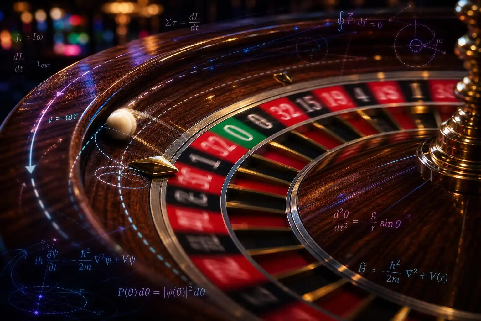
And the next time your computer shuffles a playlist or a casino claims their roulette wheel is “truly random,” you’ll know the real story: randomness is a spectrum, from the merely complicated to the genuinely irreducible, and the mathematics of that spectrum is one of humanity’s most powerful tools for making sense of an uncertain world.


Leave a Reply