

Somewhere right now, a delivery truck is threading its way through a city, hitting seventeen stops in an order that saves forty minutes of driving. A nutritionist’s app is quietly selecting which foods to recommend so that a patient hits every vitamin target while staying under a calorie limit. A rocket engineer is computing the precise burn angle that gets a spacecraft to Mars while using the least possible fuel. These problems look wildly different on the surface. Under the hood, they are all the same problem: optimization — the mathematics of finding the best possible answer within a set of constraints.
It is one of the most useful branches of mathematics you have probably never formally studied, and once you see how it works, you will start spotting it everywhere.
What Does “Optimize” Actually Mean?
In everyday language, “optimize” is a buzzword that means roughly “make better.” In mathematics, it means something precise: find the input that produces the maximum or minimum value of a particular function.
That function is called the objective function — it is the thing you are trying to maximize (profit, fuel efficiency, happiness) or minimize (cost, time, error). The inputs are the variables — the knobs you are allowed to turn. And the rules you have to obey are the constraints — the walls you cannot walk through.
Put those three pieces together and you have an optimization problem.
A tiny example: You are building a rectangular garden against a wall of your house. You have 30 meters of fencing, and you only need to fence three sides (the wall handles the fourth). What dimensions give you the largest possible garden?
Let the two sides perpendicular to the wall each have length x, and the side parallel to the wall have length y. The constraint is that you only have 30 meters of fence:
2x + y = 30
So y = 30 − 2x. The area you want to maximize is:
A = x · y = x(30 − 2x) = 30x − 2x²
This is a downward-opening parabola. Its maximum is at the vertex. You can find it with calculus (take the derivative, set it to zero) or with algebra (the vertex of ax² + bx + c is at x = −b/2a):
x = −30 / (2 · −2) = 30/4 = 7.5 meters
So y = 30 − 2(7.5) = 15 meters, and the maximum area is 7.5 × 15 = 112.5 square meters.
If you had guessed 10 × 10 = 100 square meters, you would have been 12.5 square meters short — more than the size of a small bedroom. The math found something your intuition missed.
The Calculus Connection: Following the Slope to the Peak
For smooth, continuous functions — curves without sudden jumps or corners — calculus gives us a beautiful tool for optimization. The derivative of a function tells you its slope at every point. At a maximum or minimum, the slope is exactly zero: the curve has flattened out, neither climbing nor falling. So to find the best point, you:
- Write down your objective function.
- Take its derivative.
- Set the derivative equal to zero and solve.
- Check whether you found a maximum or a minimum (the second derivative test tells you: if the second derivative is negative, you are at a peak; if positive, a valley).
This is the method behind the garden problem above, and it scales up to functions of many variables using partial derivatives — derivatives that treat all variables except one as constants, letting you find the slope in each direction independently.
The point where all partial derivatives are zero simultaneously is called a critical point, and in higher dimensions it can be a peak, a valley, or a saddle point (high in one direction, low in another — like the center of a horse saddle). Sorting out which is which is one of the central tasks of multivariable calculus.
When the Terrain Is Bumpy: Local vs. Global Optima
Here is where optimization gets genuinely tricky. The calculus method finds points where the slope is zero — but a function can have many such points. Imagine a mountain range: there are many local peaks (higher than their immediate surroundings) but only one global peak (the highest point of all). Setting the derivative to zero finds a peak; it does not guarantee you found the peak.
This distinction — local optimum vs. global optimum — is one of the central headaches of applied optimization. For some functions (specifically, convex functions, which curve like a bowl and have no local valleys except the global one), the problem disappears: any local minimum is automatically the global minimum. Convex optimization is therefore a paradise of tractability, and a huge amount of modern machine learning is built on making problems convex, or approximately so.
For non-convex problems — the bumpy mountain ranges — practitioners use tricks: start from many random initial points and take the best result, use algorithms that occasionally accept a worse solution to escape local traps (a technique called simulated annealing, inspired by how metals cool), or deploy genetic algorithms that mimic evolution, running many candidate solutions in parallel and letting the best ones “breed.”
Linear Programming: The Workhorse of the Real World
Many real-world optimization problems have a special structure: both the objective function and all the constraints are linear — no squares, no curves, just straight-line relationships. This is called linear programming (LP), and it is arguably the most economically important branch of mathematics you have never heard of.
A worked example: A small bakery makes two products — croissants and muffins. Each croissant requires 2 cups of flour and 1 egg and sells for $3. Each muffin requires 1 cup of flour and 2 eggs and sells for $2.50. The bakery has 100 cups of flour and 80 eggs available each day. How many of each should it make to maximize revenue?
Let c = number of croissants, m = number of muffins. The problem is:
Maximize: 3c + 2.5m
Subject to:
- 2c + m ≤ 100 (flour constraint)
- c + 2m ≤ 80 (egg constraint)
- c ≥ 0, m ≥ 0 (can’t make negative pastries)
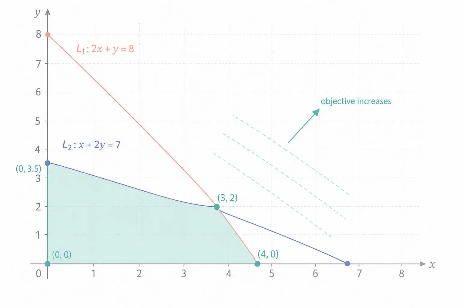
The constraints carve out a region in the c-m plane called the feasible region — the set of all production plans the bakery can actually execute. A fundamental theorem of linear programming says the optimal solution always occurs at a corner point (a vertex) of this feasible region. So you just evaluate the objective at every corner and pick the best.
The corners of this region are: (0, 0), (50, 0), (40, 20), and (0, 40).
| Corner | Revenue |
|---|---|
| (0, 0) | $0 |
| (50, 0) | $150 |
| (40, 20) | $170 |
| (0, 40) | $100 |
The answer: bake 40 croissants and 20 muffins for a daily revenue of $170 — $20 more than if you had only made croissants.
In the real world, LP problems have thousands of variables and constraints — airline crew scheduling, oil refinery blending, portfolio construction, hospital staffing. The algorithm that solves them at scale, the Simplex method, was developed by George Dantzig in 1947 and is one of the most impactful algorithms ever written. It works by hopping efficiently from corner to corner of the feasible region, always moving toward a better objective value, until it reaches the optimum.
The Traveling Salesman: When “Best” Becomes Impossibly Hard
Now for a humbling twist. Consider the Traveling Salesman Problem (TSP): a salesperson must visit n cities exactly once and return home. What is the shortest possible route?
For 5 cities, there are 12 possible routes — easy to check by hand. For 20 cities, there are over 60 quadrillion. For 100 cities, the number of routes dwarfs the number of atoms in the observable universe. No computer can check them all.
TSP belongs to a class of problems called NP-hard, where no known algorithm is guaranteed to find the exact optimal solution in a reasonable time as the problem grows. This is not a failure of cleverness — mathematicians and computer scientists have been trying for decades, and the question of whether an efficient exact algorithm exists is literally one of the most famous unsolved problems in mathematics (the P vs. NP problem, which carries a $1 million prize).
In practice, we settle for approximation algorithms that find solutions guaranteed to be within some percentage of optimal, or heuristics that work well in practice without guarantees. The routes your GPS and delivery apps compute are not always perfectly optimal — they are very good solutions found very quickly, which is often exactly what you need.
Gradient Descent: How AI Learns
Perhaps the most consequential optimization algorithm of the past decade is one you interact with every day without knowing it: gradient descent.
When a neural network learns — whether it is recognizing your face in a photo, translating text, or generating an image — it is performing optimization. The network has millions of adjustable parameters (think of them as dials). The objective function measures how wrong the network’s current answers are (this is called the loss). Training the network means minimizing the loss by adjusting the dials.
Gradient descent does this by repeatedly asking: “In which direction does the loss decrease fastest right now?” That direction is the negative of the gradient — the multidimensional generalization of the derivative. The algorithm takes a small step in that direction, recalculates, and steps again. Repeat millions of times, and the network “learns.”
The step size is called the learning rate, and choosing it is an art: too large, and the algorithm overshoots and bounces around chaotically; too small, and training takes forever. Modern variants like Adam and RMSProp adapt the learning rate automatically, and they are the reason large language models can be trained at all.
Gradient descent is not guaranteed to find the global minimum in non-convex landscapes — and neural network loss landscapes are famously non-convex, with countless local minima and saddle points. The surprising empirical discovery of modern deep learning is that it usually does not matter: the local minima found by gradient descent tend to be good enough, and in very high dimensions, most local minima have nearly the same loss value as the global minimum. The geometry of high-dimensional spaces is strange and wonderful, and it works in our favor here.
The One Insight to Carry Away
Every optimization problem, from your garden fence to a rocket trajectory to a neural network, has the same skeleton: an objective you want to maximize or minimize, variables you are free to adjust, and constraints you must respect. The mathematics gives you systematic ways to find the best answer — calculus for smooth continuous problems, linear programming for linear ones, gradient descent for the high-dimensional landscapes of machine learning, and approximation algorithms when exact answers are out of reach.
The back-of-the-envelope version of this insight is surprisingly powerful: whenever you face a decision with trade-offs, ask yourself, “What exactly am I trying to maximize? What are my real constraints?” Just naming the objective function and the constraints clearly — even without solving the math — cuts through an enormous amount of confusion. It is the first step every optimizer takes, human or algorithm.
The best answer is out there. The math helps you find it.


Leave a Reply