
There is a moment in every physics class when a student stares at a falling ball and asks: what, exactly, is its speed right now? Not its average speed over a second, not over a millisecond — but at this precise instant, when time itself has been frozen. It feels like a trick question. Speed is distance divided by time, but if no time has passed, you have zero divided by zero, which is mathematical nonsense.
That question, sitting unanswered for most of human history, is what calculus was invented to solve. And the answer turns out to be one of the most powerful ideas in all of mathematics.
The Problem With “Right Now”
Let’s make the falling ball concrete. Suppose you drop a ball from a tall building, and physics tells us that after t seconds, it has fallen a distance of:
d(t) = 4.9 × t² meters
(That 4.9 comes from half of Earth’s gravitational acceleration, roughly 9.8 m/s².)
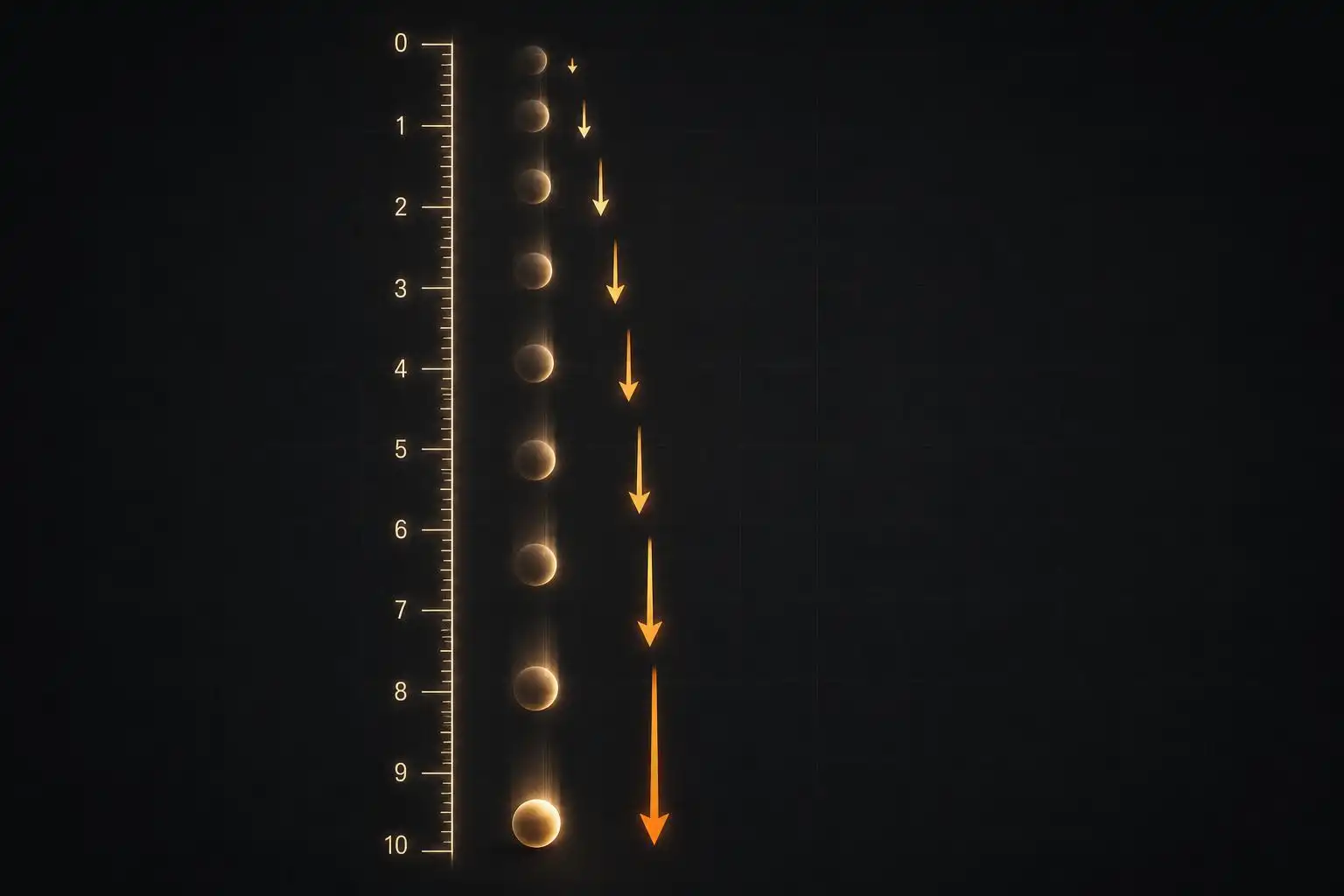
After 1 second, it has fallen 4.9 m. After 2 seconds, 19.6 m. After 3 seconds, 44.1 m. You can already feel the acceleration — the ball is covering more and more distance each second.
Now: what is its speed at exactly t = 2 seconds?
The honest approach is to measure the average speed over a short window around that moment. Between t = 2 and t = 3, the ball travels 44.1 − 19.6 = 24.5 meters in 1 second, so its average speed is 24.5 m/s. But that’s the average over a whole second — the speed was lower at the start of that interval and higher at the end.
Let’s shrink the window. Between t = 2 and t = 2.1:
- d(2.1) = 4.9 × (2.1)² = 4.9 × 4.41 = 21.609 m
- d(2.0) = 4.9 × (2.0)² = 4.9 × 4.00 = 19.600 m
- Distance covered: 21.609 − 19.600 = 2.009 m
- Time elapsed: 0.1 s
- Average speed: 20.09 m/s
Shrink it further, to t = 2 and t = 2.01:
- d(2.01) = 4.9 × (2.01)² = 4.9 × 4.0401 = 19.7965 m
- Distance covered: 19.7965 − 19.600 = 0.1965 m
- Time elapsed: 0.01 s
- Average speed: 19.65 m/s
And t = 2 to t = 2.001:
- d(2.001) = 4.9 × (2.001)² ≈ 19.61960 m
- Distance covered: ≈ 0.01960 m
- Average speed: ≈ 19.60 m/s
Do you see it? As the window shrinks toward zero, the average speed is converging — zeroing in on a single, definite number. That number is 19.6 m/s. This is the instantaneous speed at t = 2 seconds, and the process of finding it is called taking a derivative.
What a Derivative Actually Is
A derivative is the answer to the question: how fast is this quantity changing, right now?
More precisely, if you have a function f(t), its derivative at a point is the limit of the average rate of change as the interval shrinks to zero. Mathematicians write it as f'(t) or df/dt — the latter notation, invented by Leibniz, is especially evocative: it looks like a tiny change in f divided by a tiny change in t.
For our falling ball, d(t) = 4.9t², and the derivative works out to:
d'(t) = 9.8 × t
At t = 2, that gives 9.8 × 2 = 19.6 m/s — exactly what our shrinking-window calculation was converging to. The formula did in one step what we were doing by brute force.
This rule — that the derivative of t² is 2t, or more generally that the derivative of tⁿ is n × tⁿ⁻¹ — is called the Power Rule, and it’s one of the first things you learn in calculus. It’s almost magically simple. The exponent comes down as a multiplier, and the exponent drops by one.
A few more examples to build the intuition:
- f(t) = t³ → f'(t) = 3t²
- f(t) = t → f'(t) = 1 (a straight line changes at a constant rate — makes sense)
- f(t) = 7 (a constant) → f'(t) = 0 (something that never changes has zero rate of change — also makes sense)
The Geometric Picture
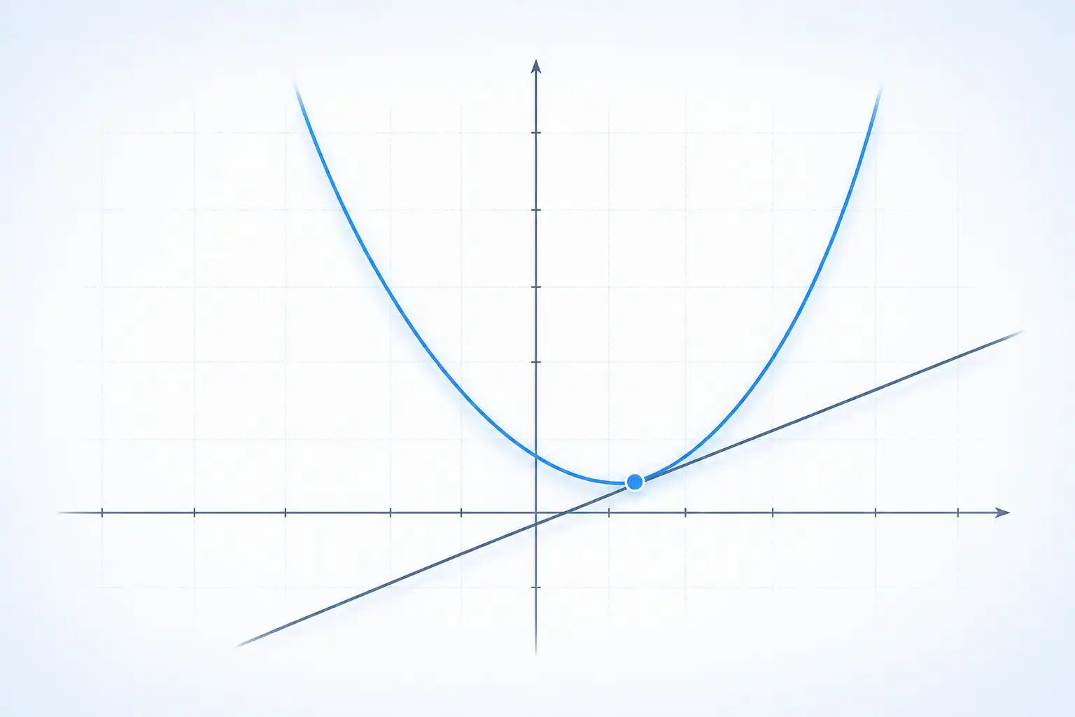
There is a beautiful way to see derivatives without any algebra at all. Draw the graph of a function — any curve. Pick a point on it. Now draw the straight line that matches the curve’s direction at that point. That line is called the tangent line.
The slope of that tangent line — rise over run — is exactly the derivative at that point.
This is why derivatives and slopes are the same thing. When the curve is rising steeply, the tangent line has a large positive slope, so the derivative is large and positive. When the curve is flat at a peak or a valley, the tangent is horizontal, slope = 0, and the derivative is zero. When the curve falls, the derivative is negative.
That last observation is more than a curiosity. It’s the key to one of calculus’s most practical superpowers: finding maxima and minima. Wherever a differentiable function hits a highest or lowest point in the interior of its domain, the derivative is zero; endpoints and constrained boundaries have to be checked separately. So to find the best or worst value of almost anything — maximum profit, minimum cost, optimal angle, peak efficiency — you often set the derivative equal to zero and solve. This is the engine behind much of modern optimization.
The Other Half: Integration
Calculus has a twin operation called the integral, and the relationship between the two is one of the most stunning theorems in mathematics.
Here is the question an integral answers: if you know how fast something is changing at every moment, can you recover how much it has changed in total?
Think of it this way. You’re driving, and you watch your speedometer the whole time. At the end of the trip, can you figure out how far you traveled? Yes — loosely, you multiply speed by time. If you drove at a constant 60 km/h for 2 hours, you covered 120 km.
But what if your speed varied continuously? Then you break the trip into tiny slices, approximate the distance covered in each slice as (speed at that moment) × (tiny time interval), and add them all up. As the slices get infinitely thin, this sum becomes an integral — written with the elongated S symbol ∫ that Leibniz chose to suggest a sum.
The breathtaking fact, called the Fundamental Theorem of Calculus, is that differentiation and integration are closely related inverse operations. The derivative of an integral gives you back the original function, under the usual conditions. A definite integral of a derivative gives the net change over an interval, and an indefinite integral of a derivative gives you back the original function up to an additive constant. They undo each other much like multiplication and division do — except they operate on functions and rates of change rather than on plain numbers.
For our falling ball: the derivative of the position function d(t) = 4.9t² gives the velocity v(t) = 9.8t. And if you integrate the velocity function v(t) = 9.8t, you get back 4.9t², up to an additive constant fixed by the starting position. The circle closes perfectly.
A Real-World Example: Maximizing a Garden
Let’s put this to work with a problem that has nothing to do with physics.
You have 40 meters of fencing and want to enclose a rectangular garden against a wall (so you only need fencing on three sides). What dimensions give you the largest possible area?
Let the side perpendicular to the wall have length x meters. You need two of those sides, plus one side parallel to the wall. So:
2x + (length parallel to wall) = 40
→ length parallel to wall = 40 − 2x
The area is:
A(x) = x × (40 − 2x) = 40x − 2x²
Now take the derivative:
A'(x) = 40 − 4x
Set it equal to zero (because the maximum occurs where the slope is flat):
40 − 4x = 0
→ x = 10
So the sides perpendicular to the wall should be 10 meters, the side parallel to the wall should be 40 − 20 = 20 meters, and the maximum area is:
A(10) = 10 × 20 = 200 square meters
Without calculus, you’d have to guess and check. With calculus, one derivative and one equation hands you the answer directly. And the same technique — find the function, differentiate, set to zero — works for engineering, economics, biology, machine learning, and anywhere else humans are trying to make something as good as it can possibly be.
Why the Universe Seems to Speak This Language
Here is the philosophical punch line, and it’s a genuine mystery.
Isaac Newton didn’t develop calculus merely because it was elegant. He developed his method of fluxions independently around the same period that Leibniz developed calculus, because the laws of nature are written in derivatives. His second law of motion (F = ma) says that force equals mass times acceleration — and acceleration is the derivative of velocity, which is itself the derivative of position. The law literally is a statement about rates of change.
Maxwell’s equations, which describe all of electricity and magnetism, are four equations in derivatives. Einstein’s field equations of general relativity, which describe how mass curves spacetime, are equations in derivatives. The Schrödinger equation, which governs quantum mechanics, is an equation in derivatives. Essentially every fundamental law of physics is a differential equation — a statement about how quantities change relative to each other.
This is strange and wonderful. The universe didn’t have to work this way. It could have been governed by rules that had nothing to do with rates of change. But it isn’t. Change begets change, and the mathematics of change — calculus — is the grammar in which nature chose to write.
The Usable Insight
You don’t need to memorize the Power Rule to carry something valuable away from calculus. Here is the mental model:
A derivative is a rate of change. An integral is an accumulation. And the two are inverse operations, with the usual constants and endpoints accounted for.
Whenever you see something changing — a stock price, a temperature, a population, an energy level — calculus is the tool that lets you ask: how fast is it changing right now? When is it changing fastest? When does it peak? How much has it changed in total?
The next time you see a curve — on a graph, on a hill, on a wave — you can picture the tangent line grazing it at every point, its slope rising and falling, telling the story of how fast the world is moving. That’s not just mathematics. That’s the shape of change itself.


Leave a Reply